The initial simulation run with the parameters determined by the initial model. The inlet pressure and the error residuals were monitored as the simulation converged.
Residual analysis
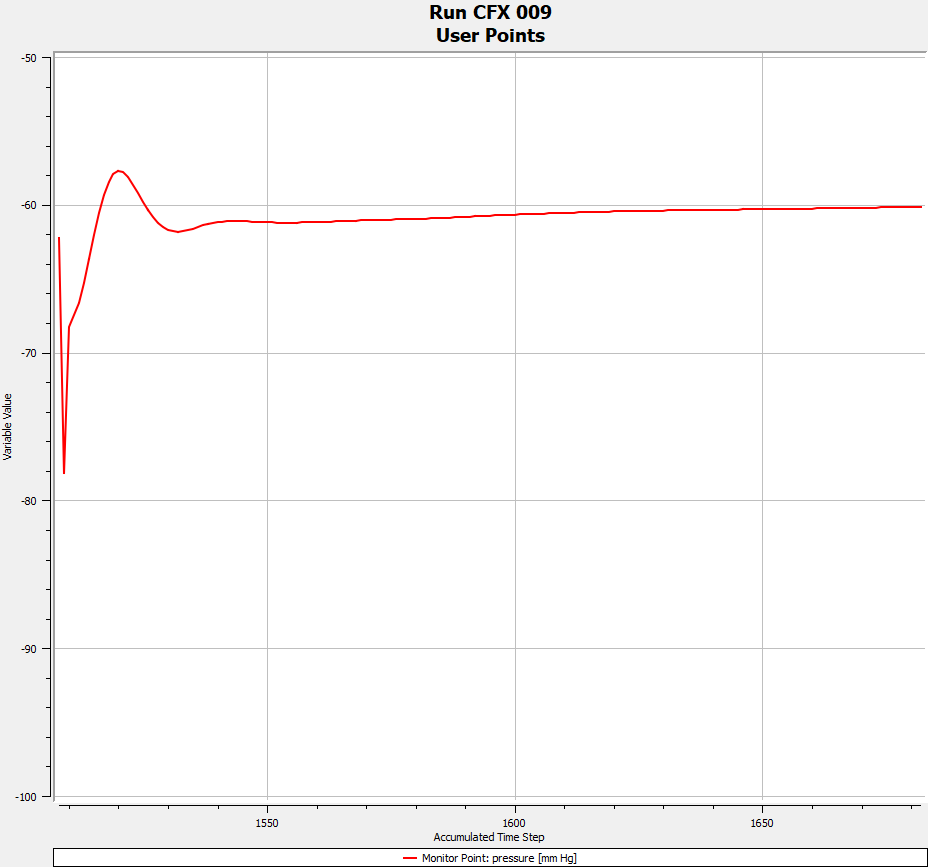
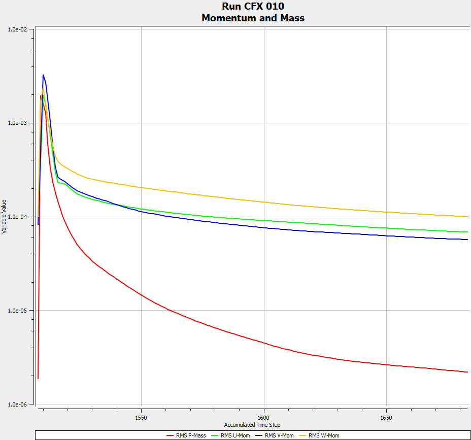 The inlet pressure (top) and momentum error residuals (bottom) plots from Ansys CFX. Note that this run was started at the 1508th timestep, and ran for 176 timesteps in total.
The error residuals fell below the 1e-4 tolerance after 176 timesteps. The inlet pressure did not change significantly after approximately 150 timesteps, so this error tolerance was suitable for the project simulations. Furthermore, the maximum number of timesteps was set to 500 to allow for slower simulations to converge successfully.
The inlet pressure may not have fully converged, as continuing the simulation revealed that the pressure slowly continued to increase. However, it did not increase significantly (a 1% change over the next 100 iterations), and a much larger number of iterations was required to show further convergence. This may have been because the simulation was run as steady-state, but the problem was inherently transient due to the rotating impeller. As there were many simulations and limited time, the original error tolerance and timestep limits were maintained.
The gradient of the residuals was relatively low indicating slow convergence. This was a sign that the timescale used to solve the problem may have been too small. Therefore, the timescale factor was increased to 1.2 making the simulation converge faster.
Velocity streamlines
Plotting velocity streamlines for the model confirmed that flow passed through the impeller and diffuser geometries to the outlet successfully. The velocity was greatest as it travelled through the inlet of the diffuser. At this point the flow had been accelerated by the impeller and was forced through the small gap ahead of the diffuser blade, leading to the high velocity. Most of the fluid passed through the diffuser, but a small amount remained trapped.
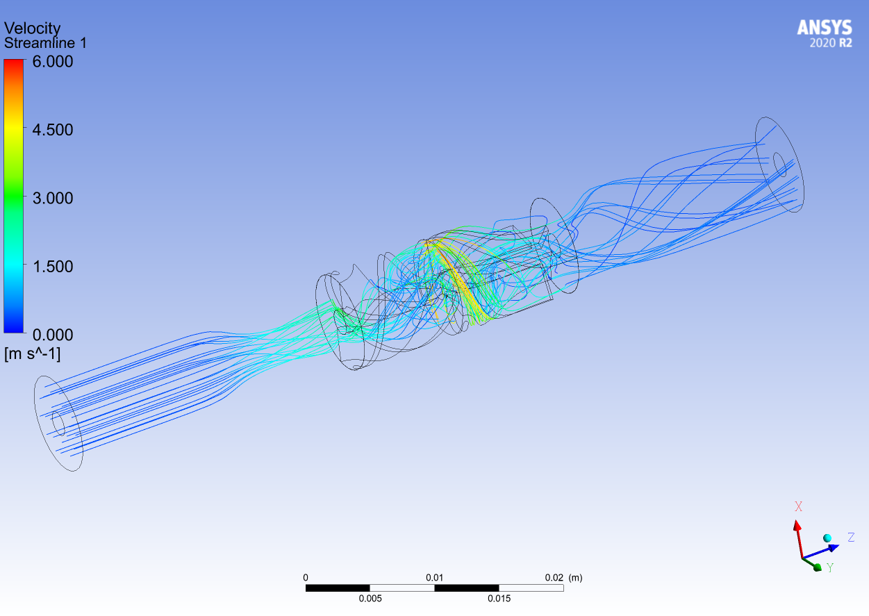 Velocity streamlines for the initial simulation.
It also confirmed that the inlet length was suitable for the flow to develop and enter the impeller. At the outlet, the flow had largely settled with minimal variations in velocity.
The streamlines verified that all domains were interfaced correctly, and there were no major issues with the prescribed flow rate at the inlet boundary, the rotational speed of the impeller, or the overall dimensions of the model.
Pressure contour
A pressure contour plot along the cross-section of the geometry demonstrated the pressure increase in more detail
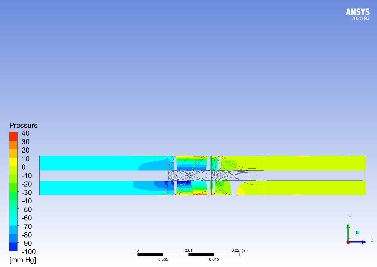 The pressure contour plot of the initial simulation.
The pressure increased from -60.3 mmHg at the inlet to the prescribed pressure of 0 mmHg at the outlet. Just before the fluid entered the impeller, its velocity increased as it was drawn in, causing a pressure drop.
The impeller domain showed pressure gradients of up to 140mmHg between the impeller hub and shroud. This may be from fluid being pushed outwards to the walls of the impeller causing high pressure. The fluid then entered the diffuser which reduced the fluid velocity causing an increase in pressure.
Limitations
The overall pressure increase was just 0.5% greater than the expected value from the operating conditions of 60 mmHg. However, there were many simplifications made to the geometry to reduce computational time. The main assumption was that the fluid inlet and outlet domains were simple pipes. The actual geometry was more complicated as fluid entered laterally through inlet windows. Additionally, the simulation was run as steady-state, so did not account for any transient blade effects.
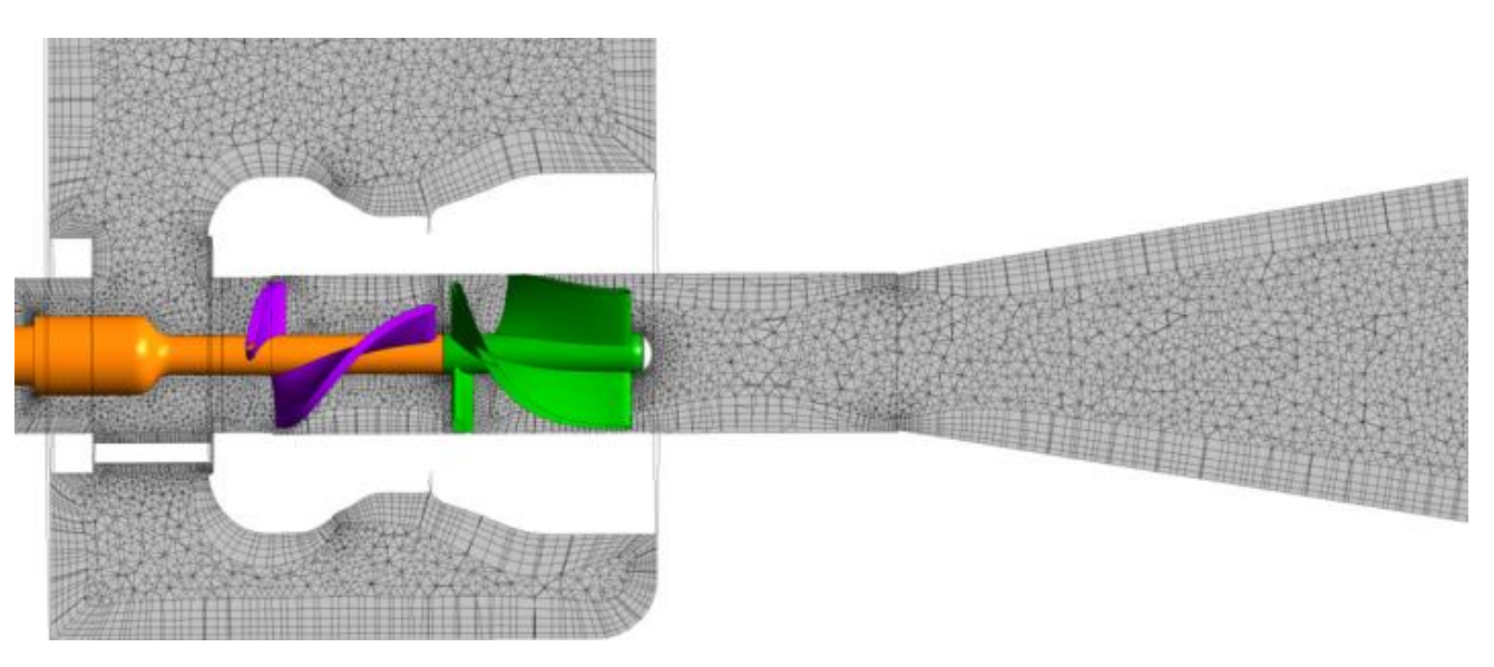 A more detailed mesh of the flow through the NeoVAD impeller and diffuser (24]).
For more reliable verification, the CFD must be compared with a more accurate model and experimental data. The project was conducted early in the design stage, so the experiments had not yet been conducted for the impeller designs.